← Blog

🌲 Finding the Trees

I built a tree detector, scored it against 450 trees whose exact positions I knew, and wrote the numbers down feeling pretty good about myself. Then I spent a week finding out what they actually meant. Three of the four were lying.

Fly a laser over a forest and it comes back with a few million points, each one an elevation where the beam hit something. Subtract the ground and what is left is the canopy — a raster of how tall the trees are. Tree tops are the high points on that surface. So you smooth it a little, look for pixels taller than everything around them, and there are your trees.

That is the whole idea. It is about forty lines of Python, it is what everybody does, and on my first real test it handed me numbers I wrote down immediately: 78.4% recall, 98.6% precision, height error of 0.44 meters — scored against 450 trees whose exact positions I knew, because I had put them there myself.

Good afternoon’s work. I was pleased. I should not have been.

Some background on why I was doing this at all. I have spent years in GIS working with rasters and vectors and things that arrive already tidy. Point clouds were the gap — a whole discipline sitting one step upstream of everything I already knew, and I had never properly gone there. So this was a stretch project: pick something genuinely unfamiliar, build the whole chain end to end, and find out where I was wrong. It turns out I was wrong in more interesting ways than I expected, which is the best possible outcome and does not feel like it at the time.

What follows is the week I spent taking those numbers apart. Three of them turned out to mean something other than what they looked like. The fourth — the one I had barely glanced at, sitting in a column off to the right — was the only one telling the truth the whole time.

The StackWhat this was built on

Before the story, the tooling, because a few of these choices did real work.

Act OneA forest I made up

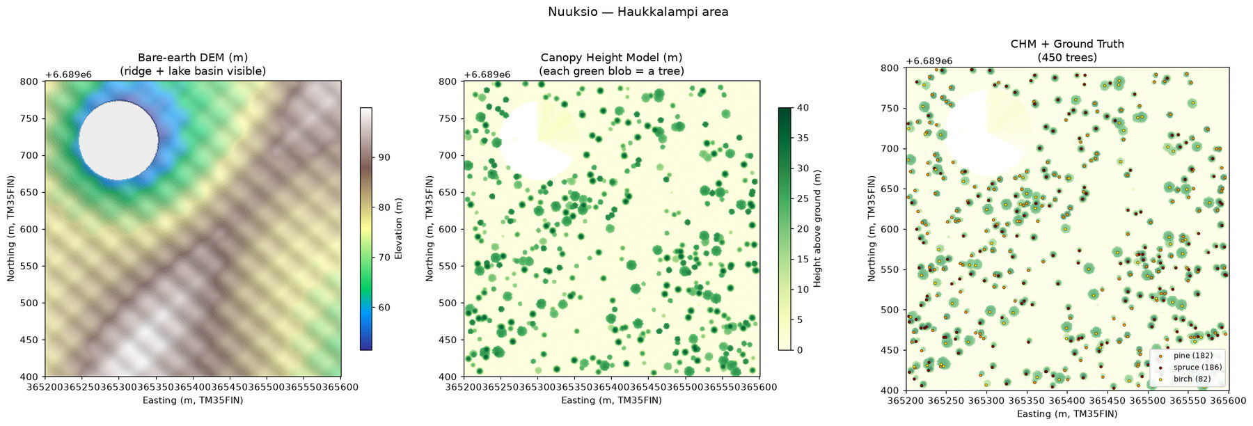
Here is the catch with measuring a tree detector: you need to already know where the trees are. Nobody hands you that for real forest — going out and surveying every stem across four hectares is somebody’s entire summer. So I built a forest instead: a boreal stand modelled on Haukkalampi in Nuuksio National Park, north-west of Helsinki. Just over a million points across 405 by 403 meters — 6.34 points per square meter — with 450 trees of known position, height and species. 186 spruce, 182 pine, 82 birch. Fixed seed, fully reproducible.

The pipeline ran clean. PDAL separated ground from canopy, produced a bare-earth DEM and a canopy height model, and the detector went to work.

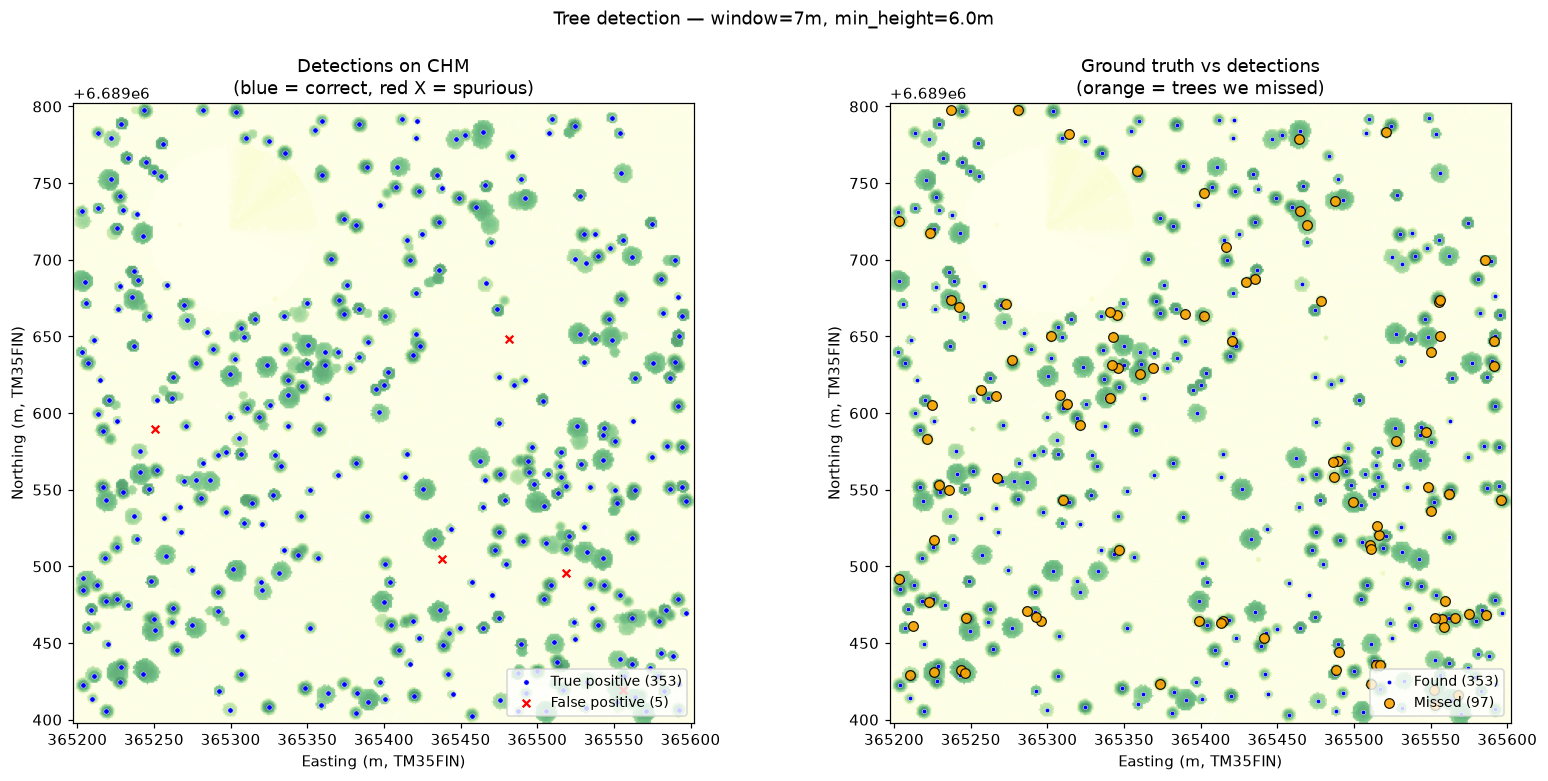
Recall by species came out in exactly the order the literature predicts. Spruce at 88.2% — tall narrow cones, easy targets. Pine at 73.1%. Birch at 68.3%, because a wide flat birch crown looks less like a peak and more like a plateau.

It was a good afternoon. I loaded the detections into Snowflake as GEOGRAPHY points, ran some spatial SQL, and got a small satisfying confirmation that the plumbing was sound:

-- stem density on a 50 m grid, over a 400 m plot
occupied cells:  62
densest cell:    56 stems/ha

Sixty-two occupied cells. A 400-meter plot on a 50-meter grid is exactly 64 cells, and two came back empty — the lake. The SQL had independently found the water body. Small thing, but it is the kind of thing that tells you the coordinates survived the round trip.

Act TwoThe number that went the wrong way

Then I went looking for trouble on purpose.

The question I actually wanted answered was how much LiDAR you really need. Finland publishes free canopy data at 0.5 points per square meter. My sample was 6.34 — thirteen times denser. Real-world data is going to be thinner than my sandbox. So how badly does this fall apart as the points run out?

Because I had ground truth, I could measure it directly rather than guess. Decimate the cloud to 0.5, 1, 2 and 4 points per square meter. Rebuild the canopy model at each. Re-score against the same 450 trees. Hold the forest constant, vary only density.

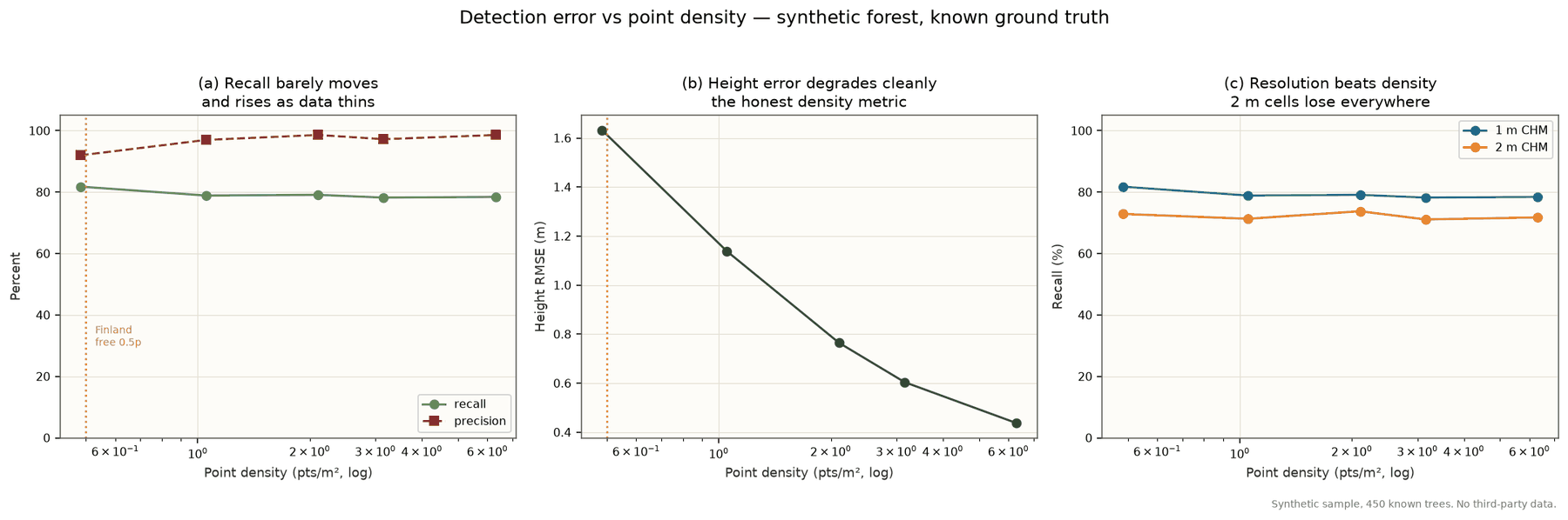
Recall went up.

pts/m²	recall	precision	false pos	height RMSE
0.49	81.8%	92.0%	32	1.63 m
1.05	78.9%	97.0%	11	1.14 m
2.10	79.1%	98.6%	5	0.76 m
3.16	78.2%	97.2%	10	0.60 m
6.31	78.4%	98.6%	5	0.44 m

At half a point per square meter a one-meter canopy raster has more empty cells than filled ones. Missing data gets written as zero. The surface becomes a field of isolated spikes separated by artificial valleys, and that roughness manufactures extra local maxima. Some of them, by luck, land near real trees. Recall rises.

Meanwhile precision falls from 98.6% to 92.0%, false positives go from 5 to 32, and height error quadruples.

F1 hid all of it: 86.6 at the worst density against 87.4 at the best.

A second result fell out of the same experiment, and it surprised me more: the 2-meter canopy model lost to the 1-meter model at every density, with birch degrading worst. Resolution was the binding constraint, not point count. Coarse max-aggregation merges adjacent crowns, and wide flat crowns are exactly what gets merged.

Act ThreeGetting out of the sandbox

Synthetic data has a ceiling, and I had hit it. My invented stand worked out at roughly 28 stems per hectare — crowns barely touching, every tree standing in its own personal clearing. I had built the easy case and then congratulated myself for solving it. Time to go find forest that did not care about my feelings.

Finland turned out to be the right answer, though not for the reason I expected.

The famous Finnish 5-point LiDAR is not free. It requires payment and Finnish strong authentication — bank credentials or a national mobile certificate — which as an American I cannot obtain at any price. The genuinely open product is thinned to 0.5 points per square meter, which my own density study had just shown is where height error goes bad.

But the Finnish Forest Centre publishes something better for my purposes: finished canopy height models derived from that licensed data, at one meter, openly licensed, no registration. And alongside them, the actual forest inventory — 1,840 stand polygons for my map sheet, with measured heights, basal areas, species composition, and a professional management plan listing which stands foresters intend to cut between 2026 and 2035.

Real ground truth. Not mine. And a published index with direct download URLs and per-tile statistics, so fetching became a database query rather than a scraping exercise:

python fetch_metsakeskus.py --sheet L4132D --year all --list

  file                           year     MB  mean_h  max_h
  ----------------------------------------------------------
  CHM_L4132D_2008                2008   59.6    9.78  39.25
  CHM_L4132D_2015                2015   68.2   12.25  39.85
  CHM_L4132D_2020                2020   55.0   12.37  41.95

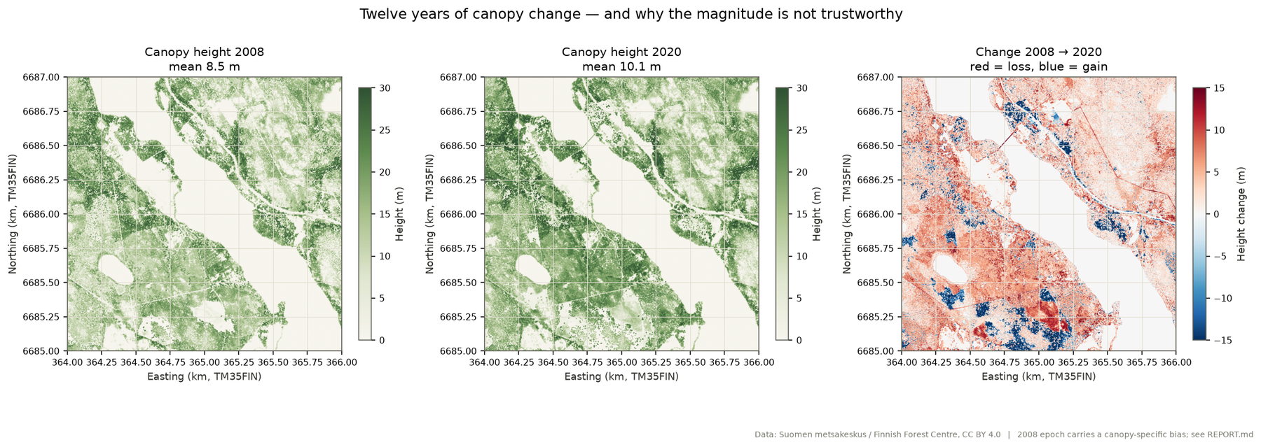
Three epochs of the same six-kilometer sheet. Twelve years of canopy change over 3,600 hectares, at one-meter resolution, free.

Act FourA bias that hid behind perfect calibration

Look at those three mean heights again. 9.78 meters in 2008. 12.25 in 2015. 12.37 in 2020.

Two and a half meters of growth in seven years, then twelve centimeters in five.

Boreal forest does not do that. Boreal forest does not do anything that dramatic; it is famously, gloriously slow. Something in my data was wrong, and it took me most of a day to work out that the something was not the forest.

My first thought was harvest, but harvest in the second period was 3.6% of the sheet against 2.6% in the first — nowhere near enough to cancel growth. My second thought was calibration, so I wrote a check: find pixels that were bare ground in the earlier epoch and compare them across flights. Ground is ground. It should read zero in any survey, and any systematic difference is the instrument, not the trees.

The ground offset came back +0.00 meters. All three epoch pairs. Perfect agreement.

I took that as reassurance. It was not. My check verified ground calibration and was structurally incapable of saying anything about canopy.

The check passed. The check was answering a different question than the one I was asking it.

What worked was stratifying the change by tree size. Real height growth falls off steeply as trees get big — a young stand adds half a meter a year, a thirty-meter spruce adds perhaps a tenth. So bin pixels by starting height, and if the growth rate does not decline across those bins, something is wrong.

There is a trap here, and I walked straight into it. If you bin by the same measurement you are differencing, you get regression to the mean: a pixel lands in the tall bin partly because noise pushed it up, and that noise does not repeat, so it drifts down on remeasurement regardless of biology. My first run produced a textbook decay curve. I believed it.

Having three epochs, I could define the bins from the middle one, whose noise is independent of both endpoints. Redone properly:

Change 2008 → 2020, binned on the independent 2015 epoch

   3-8 m     +0.247 m/yr
   8-15 m    +0.319
  15-22 m    +0.296
  22-28 m    +0.263
  28-60 m    +0.308   ← should be near zero

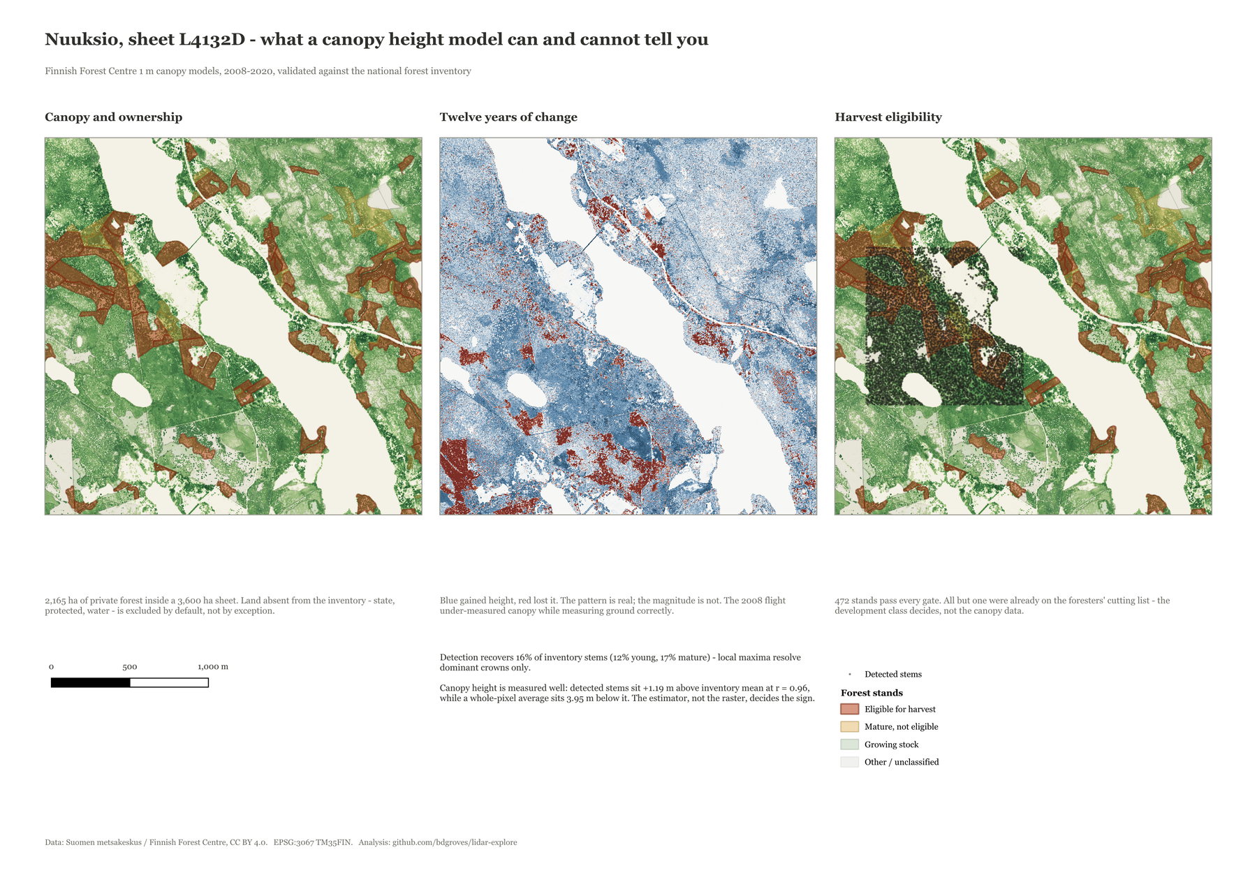
Flat. Trees thirty meters tall apparently growing as fast as trees eight meters tall, which does not happen. A constant gain independent of tree size is not growth — it is an additive offset. The 2008 flight measured canopy low while measuring ground correctly.

Act FiveThe referee arrives

Then the part I had been building toward: checking detection against an inventory measured by people standing in the forest.

This meant learning a relational schema with several traps in it, and I want to name them because each would have produced confident, plausible, wrong numbers:

Schema property	Consequence if missed
type 1 = observed, 2 = 2026, 3 = 2036	compare a raster to a simulation
summaries exist only for types 2 and 3	observed data is in strata instead
stemcount is null in strata	derive from basal area and diameter
observation dates span 1999–2024	21 years of growth reads as error
A0 and T1 attributes flagged unusable	compare against numbers the producer disowns

That fourth row cost the most and paid the most. Filtering to stands measured within six years of the canopy scan dropped 219 of 1,779 stands — and raised my height correlation from 0.907 to 0.962. Twenty minutes of date filtering bought more accuracy than any tuning I did to the detector.

I also had to correct myself on a figure I had been repeating for days. I kept saying Finnish forest runs 800 to 1,500 stems per hectare. The inventory says the median is 496, and 444 in mature stands. My number was for young unthinned forest, not forest at rotation age.

Against the real figure, the detector recovers 16% of stems. One in six.

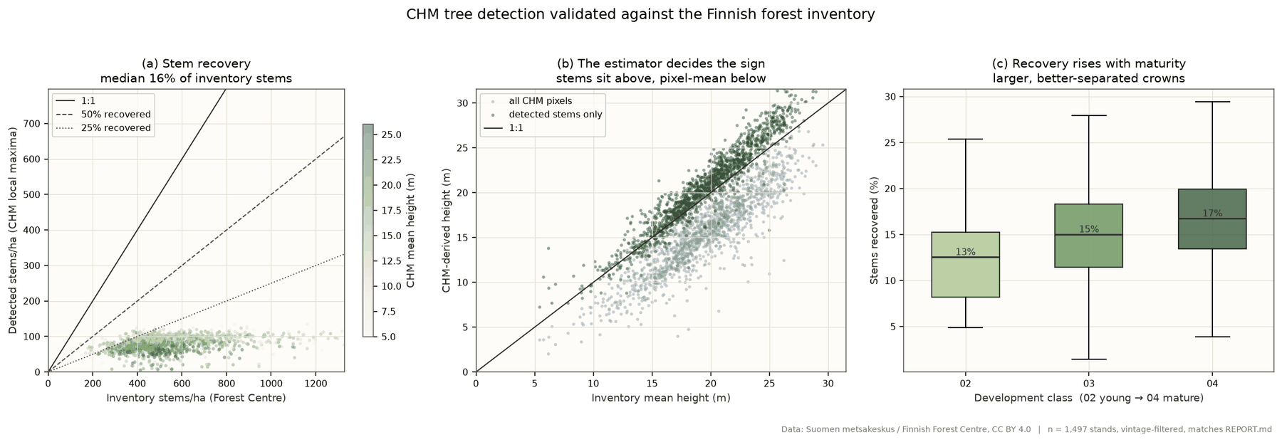
That 16% sounds bad until you see how it distributes:

Development class	inventory	detected	recovered
02 — young thinning	817	87	12%
03 — advanced thinning	635	87	15%
04 — regeneration-mature	444	70	17%

Monotonic with maturity. As stands age and thin, crowns get bigger and further apart, and more of them resolve. That is not noise — that is the physics of the method showing up across 1,295 real stands. A canopy model sees the overstory. Everything suppressed beneath it is invisible, and no cleverness in the peak-finder changes that.

And then the result I actually care about. I compared canopy heights two ways without thinking much about it, and got opposite answers:

detected stems only    20.83 m   (+1.19 above inventory)   r = 0.962
inventory mean          19.64 m
all CHM pixels          15.69 m   (−3.95 below inventory)   r = 0.901

They bracket the truth. Which makes sense once you see it: detected stems are crown apexes, so they sit above a stem-weighted mean that includes shorter trees. The whole-pixel average sits below because it includes canopy gaps — about one pixel in ten is a hole.

Same raster. Same forest. Two reasonable definitions of “mean canopy height”, five meters apart, on opposite sides of the truth.

Act SixThe result I nearly didn't report

Last piece. The inventory includes a real management plan — 5,059 operations proposed for 2026 to 2035 — so I could score my harvest ranking against decisions professional foresters had already made. This was going to be the payoff: my algorithm agrees with the experts.

It did. Fifteen out of fifteen. Precision 100%.

And it means nothing.

Because once you filter stands to development class 04 — uudistuskypsä, literally “regeneration-ripe”, a forester's own judgement that a stand has reached rotation age — 471 of 472 eligible stands were already on the cutting list. The base rate in my candidate pool was 100%. Lift over random: 1.00×.

I could not have been wrong. The classification did all the work; the expensive remote sensing added nothing on top of it.

There is a version of this project where I skip that check, publish the 100%, and it sounds tremendous. The check took twenty minutes and turned a headline into a caveat.

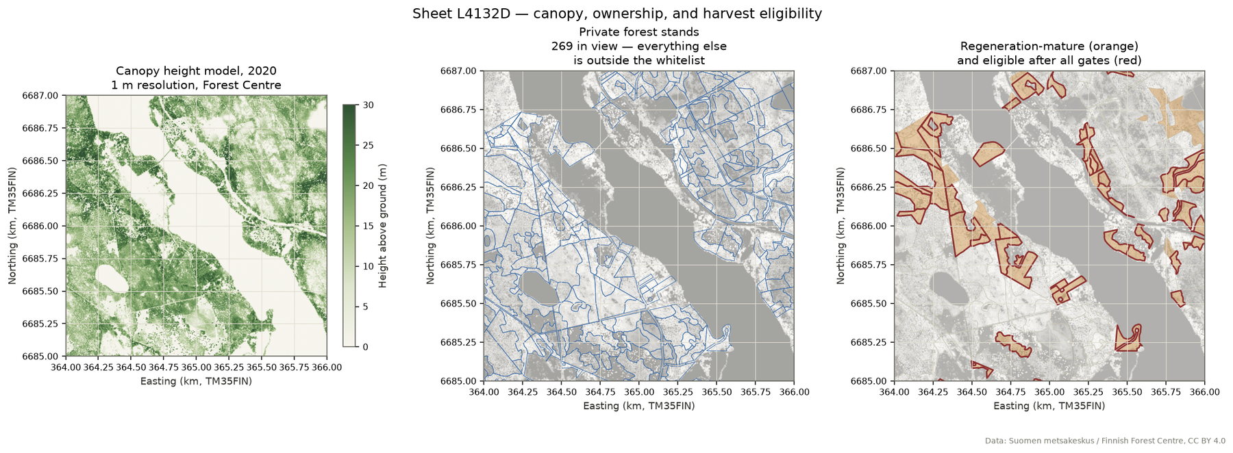
That whitelist deserves a note of its own. The inventory covers private forest. State land — including Nuuksio National Park — is administered separately and simply is not in the file. So I inverted the safeguard: rather than excluding stands that intersect protected polygons, only stands present in the inventory are eligible. Absence blocks rather than permits.

This matters because of something the algorithm did on its own. Ranking by maturity and slow growth, it walked steadily north across the sheet — toward the national park. Of course it did. Protection is what leaves forest mature and slow-growing, which are precisely the properties it was rewarding. An unconstrained targeting system does not merely risk hitting protected land; it is drawn to it.

PostscriptOne more silent failure

Right at the end, building the cartography, QGIS reported a successful table join between the stand polygons and my validation results. The fields appeared. The map rendered.

The values were shifted by two columns. det_stems_ha was returning chm_mean_h. eligible was returning obs_gap. A known quirk when you restrict a join to a subset of fields — and utterly invisible unless you happen to check a value you already know.

I caught it because I spot-checked one stand against the CSV row I had been staring at all week. Had I not, I would have published a beautiful map of the wrong thing.

Every failure in this project was silent. Not one of them threw an error.

What I'd tell someone starting thisLessons

1. Report the metric that degrades honestly. Recall improved as my data got worse. If a metric can be gamed by noise, it is not measuring data quality — it is measuring how much noise you have.
2. Check calibration on the thing you are measuring. Perfect ground agreement told me nothing about canopy and nearly reassured me into a wrong conclusion. A passing check is only as good as the question it asks.
3. Watch for one-sided sanity checks. Mine flagged implausibly fast growth and sailed past mature forest apparently shrinking, because I had written a ceiling and no floor.
4. Say which estimator produced your number. Two defensible definitions of “mean canopy height” differed by five meters and fell on opposite sides of the truth.
5. Score against the pool you actually chose from. Almost every inflated accuracy claim I have seen — my own included — comes from a denominator that quietly includes cases the method never had to discriminate.
6. Check the vintage of your reference data. Twenty minutes of date filtering moved my correlation from 0.907 to 0.962. No modelling change came close.
7. Build synthetic fixtures with known answers to test analysis code. Four real bugs came out this way: a circular ground-offset detector, the one-sided plausibility check, the wrong denominator, and a water-filled cell that qualified as a harvest stand because I never measured what fraction of it was forest.

What it meansThe part that transfers

Commercial forestry is investing heavily in exactly this: tree-level inventory from remote sensing, feeding harvest planning and yield forecasting. The pitch is a database with a row for every tree.

Having now measured it against a national inventory, I would say the honest version is narrower and more useful. Canopy height models are excellent at height and area-based structure — 1.2 meters and r = 0.96 against field-measured stands is genuinely good, and it scales to millions of hectares for the cost of a flight. They are poor at counting individual stems, and the shortfall is not a tuning problem. It is the physics of looking down at a closed canopy.

Which is precisely why Finland's national inventory runs on the area-based approach — predicting stand attributes from height distributions rather than finding individual trees — on data thinner than anything I tested. They arrived there decades ago. My density study rediscovered the reasoning from the wrong end.

And the harvest benchmark said something about where value actually sits: a forester's development-class call already determined the cutting list. If remote sensing is going to earn its cost, it will be somewhere that classification cannot reach — detecting change since the last inventory, flagging stands whose stocking no longer matches their record, catching partial cuts nobody reported. Not re-deriving a judgement already made.

Four numbers turned out to mean something other than they appeared: recall rising as data thinned, ground calibration passing while canopy was biased, two definitions of mean height landing on opposite sides of the truth, and a 100% precision that was structurally guaranteed. Each was checkable in twenty minutes. Not one of them announced itself. Every single one arrived wearing the costume of a good result.

I set out to learn point clouds. I did learn point clouds — PDAL pipelines, ground classification, height-above-ground, the whole chain from raw returns to a warehouse table. But the thing I will actually carry out of this is smaller and more portable than any of that: the metric that flatters you is rarely the metric that is telling you the truth. Height RMSE sat in a column I ignored for two days while I admired a recall score that got better as my data got worse.

The forest was there the whole time. Four hundred and fifty invented trees in a Finnish national park I have never visited, then 1,295 real stands measured by people who actually walked into them with calipers. It took a national inventory, built by strangers over twenty-five years and given away for free, to tell me what I had been looking at.

Worth the week.