Today Aaron Becker asked a fun question on X, under my Serpent Mound post, addressed to me and to Milos Popovic, who makes forge3d: are we using forge3d from inside notebooks, or mostly through agents?
My honest answer was agents. I describe the scene, Claude writes the forge3d script, and the heavy renders run on GitHub Actions, because my Windows laptop’s security settings won’t let freshly installed Python libraries load. It works really well. But it does mean the “how” lives in scripts and commit messages, not somewhere you can just sit and read.
So today I fixed that. Nine of my forge3d projects now have a walkthrough notebook.
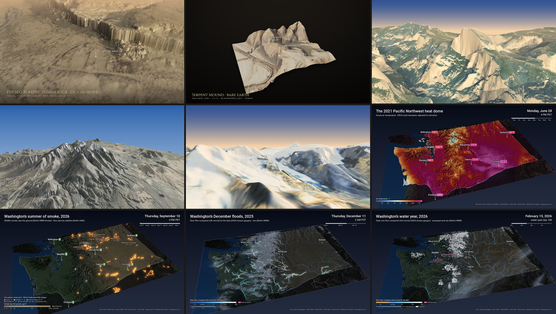
One frame from each notebook, all rendered with forge3d on a computer with no graphics card
What’s in Them
Each notebook goes from the raw data to a finished frame, in order, using the project’s own code rather than a tidied-up copy. If the notebook shows a step, that’s the step the real render takes. And each one is saved with its outputs, charts and renders included, so it reads like an illustrated article right on GitHub. You don’t need to install anything to follow along.
- SOLSTICE · Chaco CanyonThe Sun on the solstice mornings, Pueblo Bonito’s real skyline from lidar (it pushes the June sunrise back more than an hour), and the close-up of the great house taken apart layer by layer.
- Project Kiva · Serpent Mound2.3 million laser returns streamed out of the USGS archive, a bare-earth model, six ways of reading relief side by side, and a cross-section that shows how a metre-high mound stands out right next to a 25 m bluff.
- Yosemite Valley flyoverThe granite trick for cliffs that aerial photos can’t see, the flight drawn on a map with its speed, lens and clearance, and four frames from Half Dome to Tunnel View.
- Once around Humphreys PeakHow one slow orbit is written as keyframes, and the camera maths that lets each label land on its summit and hide when a ridge gets in the way.
- Up the Icefields ParkwayA 100 km scene from Copernicus and Sentinel-2, the fix for lakes with a ridge’s shadow lying on the water, and why this one drops the shadow map.
- The 2021 heat domeA week of hourly temperature from a 9 km grid, nudged for elevation pixel by pixel, and the green-screen trick that keeps the ocean blue.
- The summer of smoke, 2026Smoke at the cities and fire detections day by day, and the two-pass render that hides the smoke amount in the ratio of red to blue so it survives the lighting.
- The December 2025 floodsRain sweeping in and the gauges that passed their records, plotted against their old crests, then the rivers drawn by how far above normal they ran.
- The 2026 water yearA year of snowpack, rain and river flow against normal, and the same map on a February day and an August one.
Things I Noticed Along the Way
Writing a notebook is a bit like explaining a recipe to a friend: you find out which steps you’d been doing on autopilot. A few of my favourites:
The viewer’s mesh is square. forge3d’s terrain viewer builds its mesh at most 2,048 points on a side, and it reports the size in its log. My Yosemite DEM is 7,680 × 4,200 cells at 3 m, so in the film the terrain is really a point every 11 m east–west and every 6 m north–south. It’s also why SOLSTICE draws each frame in nested layers: that’s how its close-up gets true half-metre lidar.
Smoke hides in a colour ratio. Lighting changes how bright the smoke is, so the smoke project renders it twice: once as land, once as a pure red-for-smoke, blue-for-clear code. Shading scales red and blue together, so their ratio still tells you how thick the smoke was, and the finishing pass turns it back into haze.
The ocean is a green screen. Flat water comes out grey under the viewer’s lighting, so the Washington maps paint it a key green that no data colour uses, and swap it for deep Pacific blue afterwards.
Cliffs get a little help. Aerial photos are taken straight down at midday, so a 900 m wall like El Capitan is a few smeared pixels in shadow. Steep faces get a granite tone (limestone grey in the Rockies) and the evening sun does the rest.
The notebooks also caught one of my own slips. Project Kiva’s atlas was counting each site’s laser returns over a slightly bigger area than it divided by, so the “points per square metre” figures all read a little high. They’re fixed now. Serpent Mound, for example, is 6.8 per m², not 7.9.
Running Them Yourself
Each project’s README says which data to download first; most of it is one pixi command. The charts and maps need nothing special. The renders need forge3d’s viewer, which wants a graphics card, or on Linux, Mesa’s software Vulkan driver under a virtual display. That’s how every frame in this post was made: a cloud computer with no GPU, a couple of minutes per notebook. SOLSTICE and Project Kiva also have a Run notebooks button in GitHub Actions that re-runs them and saves the results.
Thanks for Asking
forge3d keeps turning into one of my favourite tools, thanks to Milos, and Aaron’s question was the push I needed to show my work. If you’ve been curious about any of these flights, now you can open the hood.
Rendering: forge3d by Milos Popovic. Data: USGS 3DEP and The National Map, USDA NAIP, Copernicus GLO-30 and Sentinel-2, ERA5-Land via Open-Meteo, NOAA HRRR and HRRR-Smoke, NASA FIRMS, NIFC, USGS Water Services, HydroRIVERS, Natural Earth.
Go deeper
Brian Granger and Fernando Perez of the IPython Project — Podcast.__init__, 13 June 2015, about 68 min. The two founders on how a better Python shell grew into the Jupyter notebook.
#44: Project Jupyter and IPython — Talk Python To Me, 2 February 2016, about 61 min. Core developers Min Ragan-Kelley and Matthias Bussonnier on notebooks, kernels and the big split from IPython.
Longtime cartographer reveals there’s more to a map than meets the eye — The Conversation (Hawaiʻi Public Radio), 5 February 2026, about 13 min. Retired National Park Service cartographer Tom Patterson on the craft of shaded relief.
Knuth, D.E. (1984). Literate programming. The Computer Journal 27(2), 97–111.
Kluyver, T., Ragan-Kelley, B., Pérez, F., Granger, B., Bussonnier, M., Frederic, J., Kelley, K., Hamrick, J., Grout, J., Corlay, S., Ivanov, P., Avila, D., Abdalla, S., Willing, C. & Jupyter Development Team (2016). Jupyter Notebooks – a publishing format for reproducible computational workflows. In Positioning and Power in Academic Publishing: Players, Agents and Agendas, IOS Press, 87–90.
Rule, A., Birmingham, A., Zuniga, C., Altintas, I., Huang, S.-C., Knight, R., Moshiri, N., Nguyen, M.H., Rosenthal, S.B., Pérez, F. & Rose, P.W. (2019). Ten simple rules for writing and sharing computational analyses in Jupyter Notebooks. PLOS Computational Biology 15(7), e1007007. Open access.
Horn, B.K.P. (1981). Hill shading and the reflectance map. Proceedings of the IEEE 69(1), 14–47.
Kennelly, P.J. & Stewart, A.J. (2014). General sky models for illuminating terrains. International Journal of Geographical Information Science 28(2), 383–406.
Zakšek, K., Oštir, K. & Kokalj, Ž. (2011). Sky-view factor as a relief visualization technique. Remote Sensing 3(2), 398–415. Open access.
Cartographic Relief Presentation — Eduard Imhof’s classic on hillshading, tints and contours, back in print from Esri Press.
forge3d — Milos Popovic’s Rust-and-WebGPU terrain renderer for Python. · Project Jupyter — the notebook format itself. · pixi — the one-command environments behind each project.
USGS 3D Elevation Program (3DEP) — the lidar under most of these frames. · Open-Meteo Historical Weather API — ERA5-Land, hour by hour, for the heat dome.
Shaded Relief — Tom Patterson’s generous home for terrain-rendering techniques and free relief art.